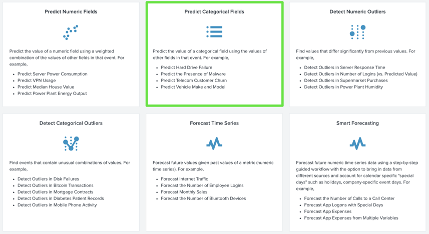
The Splunk MLTK app comes bundled with over 30 common algorithms as well as 6 'Experiment' workflows used to guide us through the pipeline of creating, testing and deploying machine learning into our Splunk environment.
Below are the workflows provided in the latest MLTK app:
In this blog, we are going to take a look at how I used the 'Predict Categorical Field' algorithm to predict what Knowledge Base (KB) articles should be assigned to ServiceNow Incidents based on previous Incident and KB relationships. We achieved this by reading and dissecting the Incident Description fields of new Incidents and comparing them against historical Incident Descriptions and their related KB articles. This allows you to predict the most effective KB article to leverage and drastically reduce mean time to incident resolution. This approach transitions ServiceNow from a passive ticketing system into a proactive recommendation engine. In the example below we analyzed 3 months worth of ServiceNow data.
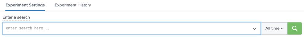
The Predict Categorical Field algorithm learns and classifies data into one category or another based on the relationships identified in the data. So how did we go about it? Within the MLTK app, under the ‘Experiments’ tab, we are presented with 6 Experiment workflows. Clicking on the ‘Predict Categorical Field box we are now in the workflow GUI.
Step 1: Search and format my data
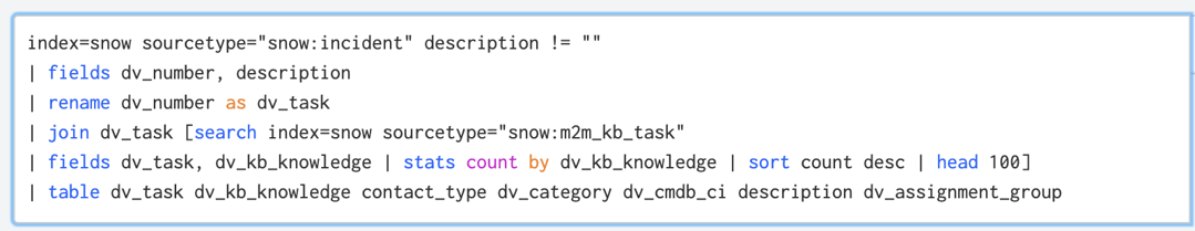
The first thing I had to do was to format the data and make it useful. In the below search, you can see I joined 2 tables, the incident table and the m2m_kb_task table, which has the KB data. You can also see I used the stats count and sort/head commands and selected the top 100 rows. The reason for this is to choose the top 100 most popular KB articles, that is, KB articles that have been assigned to a lot (i.e. ~50+) of Incidents.
For our model, we want to choose KB articles that map to the most Incidents. This helps the model learn the relationships. If we use KB articles that are only assigned to one or two rare Incident types then the model won’t work. Also, we only want to use fields in the prediction that will help, not hinder the prediction. We want to choose fields that will group or categorize our data. (i.e. contact_type, assignment_group etc.). Fields that have too many unique values will drag down your prediction accuracy.
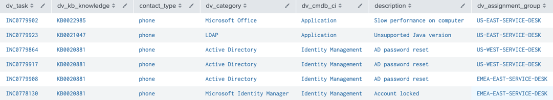
This produces the results I need to pass into the MLTK Categorical Predictor engine:
Step 2: Use processing algorithms to enhance my data. (TFIDF, StandardScalar & PCA)
Now we’re going to sprinkle some of the MLTK magic on the data and use some pre-processing algorithms to prepare our data before we use it in our model. This will provide better results in the end. To apply these algorithms we use the fit command. The first processing algorithm we used was TFIDF.
What is TFIDF I hear you ask? Well it’s a fantastic algorithm we can use to analyze text. Without getting into too much of the underlying mathematics, TFIDF (term frequency–inverse document frequency), converts raw text into numeric fields, making it possible to use that data with other machine learning algorithms. It basically weighs each text term in importance based on the frequency it appears in the text we point it at. (In our case the description field of Incidents & KB articles.)
| fit TFIDF description stop_words=english max_features=400
I used two parameters with TFIDF, 'stop_words' and 'max_features'.
Max features: This builds a vocabulary that only considers the top K features ordered by term frequency.
Stop Words: This is used to omit certain common words such as "the" or "an", or “or” :).
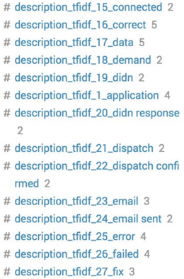
Below you can see the results. It creates new fields and assigns a numerical value to each based on the weighting.
Next up is the StandardScalar processing algorithm.
The StandardScaler algorithm uses the scikit-learn StandardScaler algorithm to standardize the data fields by scaling their mean and standard deviation to 0 and 1, respectively. This standardization helps to avoid dominance of one or more fields over others in subsequent machine learning algorithms. StandardScaler is useful when the fields have very different scales. StandardScaler standardizes numeric fields by centering about the mean, rescaling to have a standard deviation of one, or both.
| fit StandardScaler description_tfidf*
Finally we pop the results of the StandardSaclar through the PCA algorithm. The PCA algorithm uses the scikit-learn PCA algorithm to reduce the number of fields by extracting new uncorrelated features out of the data.
| fit PCA k=3 SS_*
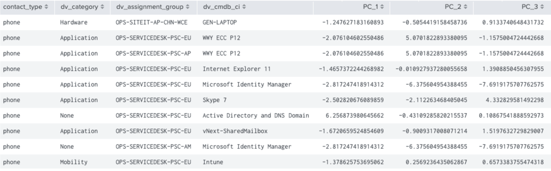
The resulting table is all the fields we need for our prediction.
You can also see in the results, the PC_1, PC_2 & PC_3 fields which are the numerical translation of our description text fields.
Step 3: Use processing algorithms to enhance my data
Now we want to feed these results into our 'Categorical Predictor' algorithm. In this case, I’m using the RandomForestClassifier algorithm. The RandomForestClassifier algorithm uses the scikit-learn RandomForestClassifier estimator to fit a model to predict the value of categorical fields.
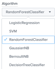
There are also other algorithms we can use instead of RandomForestClassifier. It’s worth playing around with each to see how they affect your results.
Next, we choose the field to predict and the fields we intend on using to do the predicting.
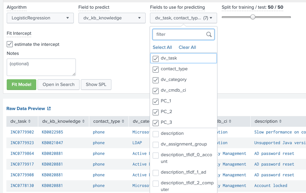
For the 'Field to predict' we choose 'dv_kb_knowledge' then we select the 'Fields to use for prediction'; In this case we choose the dv_task, contact_type, dv_category, dv_cmdb_ci and the PC_* fields which are the results of our StandardScalar algorithms above. For the 'Split for training/test:' parameter I chose 50/50. This means I’m using 50% of the data to teach my model and then the remaining 50% to predict the KB field.
Once you have everything selected, then it’s time to hit the Fit Model button!
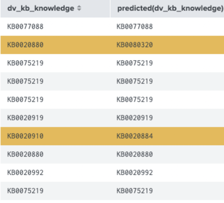
The results show us which KB articles the algorithm predicted correctly (matching value) and incorrectly (highlighted orange).
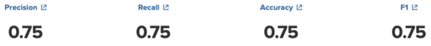
In this case we got a 75% accuracy score. That’s 3 correct predictions out of 4 which ain't bad!
To improve accuracy beyond 75%, I plan on using the Natural Language Processing (NLP) functionality next to pre-process the text, prior to MLTK using it. That way we can standardize terms similar to the way the CIM model works in Splunk. For example, the description text entered by automated systems have a finite range of possibilities, whereas text entered by humans can vary widely, and have infinite possibilities dragging our score down. Take database, data base, DB etc. for example. NLP can help with this and the success of the prediction should significantly improve.
Natural Language Processing app -> https://splunkbase.splunk.com/app/4066/
If you are planning on going down a similar route or have any questions or recommendations for improvement please don’t hesitate to reach out.
Want more insight like this? Make sure to follow us on LinkedIn, Twitter and Facebook!